Eyes, JAPAN
Demystifying Data Classification with Mathematics
Jun Wen
英語のあとに日本語が続きます。
Our modern information era is characterized, for better or worse, by a continuously-changing data science landscape, which is why it is often said around the world that any professionals in the ICT (information and communication technology) realm must embrace continuous upskilling and unlearning/relearning of techniques. For instance, programming languages can show up one day, then leave soon after – then, it behooves us to remain flexible in our ICT journey. That said, two pieces of the backbone of data science remain constant: The mathematical concepts, and the business-driven motivations behind the developments in technology. One exemplar of data science implemented into machine learning is the Support Vector Machine (SVM). Today, let us delve into the SVM as an example of the constancy of mathematics and motivations, and learn more about the “Why?” behind certain elementary mathematical ideas that are often taken for granted even by professionals.
Case study of the day: Support Vector Machines (SVMs)
At its core, a Support Vector Machine is an algorithm in machine learning that relies on “supervised learning,” which mentors a model by providing it with a training data set, like a school tutor showing a set of exercises and solutions to the class before letting them attempt their work. For supervised learning, the training set lists some inputs, and matches them with corresponding desired outputs, so that the model learns to emulate that matching process. Consequently, the model learns to match new data to specific groups as well, thus classifying data into different groups.
Indeed, for SVMs in particular, they are traditionally employed to segregate data into two distinct groups. In the modern ICT industry, this type of binary classification sees usage in categorizing documents (be they handwritten or typewritten), such as in quickly filtering out only the documents relevant to a specific company goal (Maitra et al., 2015). Another application gaining interest in recent years is using SVMs in the medical industry, such as filtering out medical image data that is sufficiently informational (Maitra et al., 2015), versus those too beleaguered by visual noise to be worth keeping.
A simple visual demonstration is given below: There are various points scattered in a space, and SVM creates a line that splits the points into two separate groups.
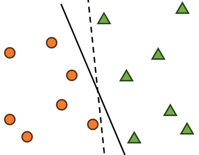
Figure 1: Examples of hyperplanes (in this case, lines) separating points into two groups.
Figure 1, while simple, shows a key challenge in the designing of SVM algorithms: There are multiple ways to separate data into two groups, just like there are multiple ways to draw the line (solid vs dotted) in Figure 1 that splits the points apart. How do we know which line is best, to ensure that new information entering our machine learning framework in the future also gets classified correctly? That is where mathematics is used to ensure that we, as users, feed the model instructions that ensure it learns the best possible method of drawing that line.
[Note 1: The “line” is actually a hyperplane. Informally it’s a flat surface that splits a space into two separate partitions, regardless of how many dimensions that space is in. I will stick to the informal word “line” for this discussion.]
[Note 2: Incidentally, there also exists multiclass versions of SVM that sort information into more than two categories, but these complex classification tasks bring a new set of challenges (van den Burg & Groenen, 2016), since it’s no longer as easy as slashing down a single line into the middle of the data points, for example. So, for the purposes of today’s discussion, we limit ourselves to the fundamentals of the easiest case scenario of traditional SVMs.]
How to make the training data set
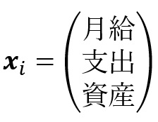
Let’s consider an example of SVM usage in the industry: Perhaps a bank (You are now a bank.) might want to measure a person’s monthly salary, monthly spending, and cash value of existing assets, and then judge if they are trustworthy, i.e. if they are acceptable clients for loaning money to. For instance, someone with few existing assets and excessive spending might not be a cooperative debtor, and is hence untrustworthy.
How do we create the training data set? Gather a list of known people (let’s say there are m people), and for each, take the numbers representing salary, spending, and assets and put them in a vector 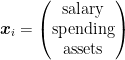

![\left \{ \left [ \boldsymbol{x}_i,y_i \right ]: 1\leq i\leq m \right \}](https://s0.wp.com/latex.php?latex=%5Cleft+%5C%7B+%5Cleft+%5B+%5Cboldsymbol%7Bx%7D_i%2Cy_i+%5Cright+%5D%3A+1%5Cleq+i%5Cleq+m+%5Cright+%5C%7D&bg=ffffff&fg=000&s=0&c=20201002)
For instance, say we have a small group of m = 3 people:
- a student with no salary nor assets, spending $2000 a month,
- a fresh graduate earning $4500 and spending $6000 a month,
- and a middle-aged worker earning $9500 and spending $6000 a month, with $40 000 of assets (e.g. investments) in this name.
We can then represent the 3 people as 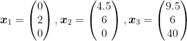

![\left \{ \left [ \begin{pmatrix}\textup{0}\\ \textup{2}\\ \textup{0}\end{pmatrix},-1 \right ], \left [ \begin{pmatrix}\textup{4.5}\\ \textup{6}\\ \textup{0}\end{pmatrix},-1 \right ], \left [ \begin{pmatrix}\textup{9.5}\\ \textup{6}\\ \textup{40}\end{pmatrix},1 \right ] \right \}](https://s0.wp.com/latex.php?latex=%5Cleft+%5C%7B+%5Cleft+%5B+%5Cbegin%7Bpmatrix%7D%5Ctextup%7B0%7D%5C%5C+%5Ctextup%7B2%7D%5C%5C+%5Ctextup%7B0%7D%5Cend%7Bpmatrix%7D%2C-1+%5Cright+%5D%2C+%5Cleft+%5B+%5Cbegin%7Bpmatrix%7D%5Ctextup%7B4.5%7D%5C%5C+%5Ctextup%7B6%7D%5C%5C+%5Ctextup%7B0%7D%5Cend%7Bpmatrix%7D%2C-1+%5Cright+%5D%2C+%5Cleft+%5B+%5Cbegin%7Bpmatrix%7D%5Ctextup%7B9.5%7D%5C%5C+%5Ctextup%7B6%7D%5C%5C+%5Ctextup%7B40%7D%5Cend%7Bpmatrix%7D%2C1+%5Cright+%5D+%5Cright+%5C%7D&bg=ffffff&fg=000&s=0&c=20201002)
Quick reminder: this often means having, using Python for example, Numpy arrays (for 
print(training_set[0])
would return
[array([[0],
       [2],
       [0]]), -1]
and
print(training_set[2][1] == 1)
would return
True
How does the SVM draw the line?
Returning to the realm of mathematics, now that a training data set has been created, the next task is to have the model learn how to draw the “line” that separates all current and future data into two groups. Mathematically, this means the model studies the training data set, then learns a function 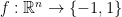
After being created via supervised learning, the model takes a new data point 


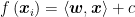
However, the function f is most commonly designed to be linear (Meyer et al., 2003), which is why we often use straight lines for dividing the points in SVMs. Mathematically, this means the score is calculated via the function 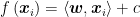


Optional section: A refresher on what the inner product is
For two vectors 

However,
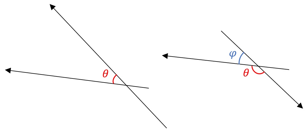
Figure 2: The angle θ between two angles can be drawn like so.
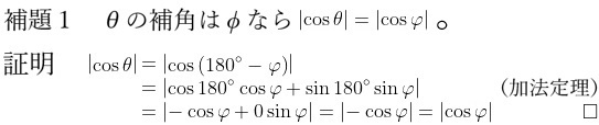
Whenever there is an angle θ, its supplementary angle φ can also be used in the inner product’s calculation, which will be proven below.
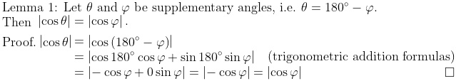
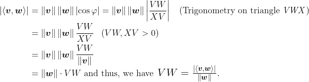
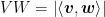
Lemma 1 allows us to calculate the lengths of the sides of right-angled triangles formed by vectors, such as the length of line segment VW in the diagram below:

Figure 3: Vector v goes from X to V, and vector w (blue arrow) is parallel to the line segment VW, which is perpendicular to line segment WX.
Referring to Figure 3, suppose we have two vectors v and w that are not parallel, so the angle between them is θ, with the supplementary angle φ. Here, v is longer than w, so we use v as the hypotenuse of the right-angle triangle VWX, where VW is purposely made to be parallel to w (so that φ is equal to the corresponding angle XVW), and WX is purposely made to be perpendicular to line segment VW. Lastly, this line segment VW is the length of the projection of v on w. It’s like how, if the sun shone directly above vector v, the shadow being casted would be the line segment VW.
Now, it turns out that 

But we know angle VWX is a right angle, so elementary trigonometry implies the following:
Of course, if the norm of w is just 


![]()
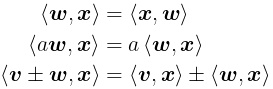
We conclude with a final remark: The standard inner product is a bilinear form, which means it follows these linearity properties below. This is helpful later, too:
What is the best line for the SVM to draw?
Now that we know the steps behind drawing a “line” for the SVM to split the data into two groups, the next question becomes, how does the machine learning model know which line is the best to use? We want to give the model instructions to ensure it chooses a line as far away from both groups of data points as possible (Figure 4, dotted line), so that we reduce the likelihood of a new data point being assigned to the wrong group. However, recall that the line is identified by the equation 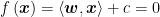

Figure 4: The best possible line (dotted) should be as far away as possible from the two groups of data points visible in your training data set. Otherwise, points like the circled one might get misclassified.
Since the trustworthiness 
Hence, the idea now is, we need to give the model instructions that let it choose the best w and c values, to ensure that when the yardsticks are drawn, the gap between them is as large as possible. That way, even if a new data point is added (the circled green point in Figure 4), we minimize the chance of misclassification. (For example, if the dividing line at = 0 is replaced with the = 1 line, then the green point ends up on the line’s LEFT side instead, where the orange points are, which is a misclassification.)
The mathematics behind identifying the best line
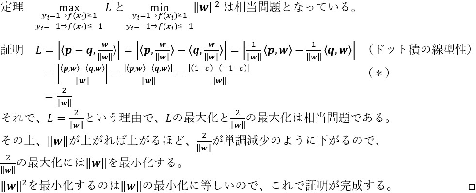
Thus, our last job is to figure out: what does, “the model must choose w and c to ensure that when the yardsticks are drawn, the gap between them is as large as possible,” mean for the instructions we give our model? Those who have studied data science will know two statements taken for granted:
- the distance between the yardsticks, regardless of dimension, is always
,
- the instruction to give the model for choosing w and c takes the form
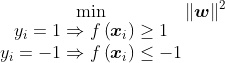 .
.
As seen above, the criteria for minimization is 
But, why does the mission of, “maximize the distance between the yardsticks” evolve into, minimize 

Figure 5: The orange distance needs to be maximized, in order to make the gap between our “yardsticks” as wide as possible. O here is the origin.
First, we set the stage: Draw in your yardsticks
Now, let p represent a position vector for any point on the yardstick
What we do know is that we defined p to point to an arbitrary position on the yardstick 

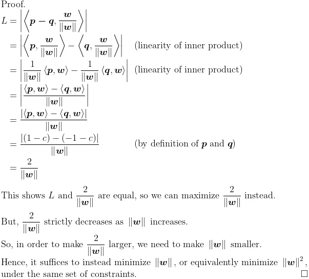
Next, we can also create a vector p – q using vector addition and subtraction. All of the objects discussed have been drawn above in Figure 5, in black. Then, to make sure the yardsticks are as far apart as possible, we need to calculate this distance L (note that L > 0), labelled in orange, and maximize it. But, L is just the projection of p – q onto w ! (Feel free to compare Figures 5 and 3 — I made Figure 5 by copy-pasting Figure 3 and then doing small edits, anyway…) Of course, by extension, this also means L is the projection of p – q onto the unit vector 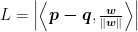
We are now ready to prove that maximizing L, the distance between the two yardsticks, is also achieved by minimizing

Since we never chose any specific point when creating p and q, the mathematical arguments above work for ANY point along the yardsticks, and therefore the entirety of both yardsticks obey the arguments presented. So, we can confidently say that the distance between the two yardsticks is  is the instruction needed by the SVM to choose the best possible w and c to make function f, so as to calculate the scores of new bank customers. In conclusion, rather than having to make your own judgment calls after studying the bank’s customers one by one, you can now make the SVM automatedly pick out exactly who can be trusted by the bank with larger and riskier loans!
Conclusion
We have, in our discussion today, covered the following points:
- What is an SVM?
- An example of using traditional SVMs in the industry
- An optional refresher course about the inner product, which is used by SVMs to draw the line (hyperplane) needed to separate data into two groups
- Two gospel truths: the distance between the yardsticks used by the SVM is
(1) learning from the training data set,
(2) obeying the instruction - Mathematical proofs behind the two truths.
However, this is barely the tip of the iceberg in terms of the underlying mathematical theories behind why SVMs or machine learning in general work. For instance, with a training data set whose data points cannot be separated by a single straight line, how do we design SVMs that use curved boundaries instead?
I want to end by leaving you with one particularly important train of thought: If it is enough to minimize 
数学でデータ分類を解明しよう 日本語版
情報化時代は、良くも悪くも日夜変化し続けるデータサイエンスの状況によって特徴付けられています。そのため、世界中でよく「ICT(情報通信技術)の分野の専門家は、継続的にスキルアップや技術の再学習を受け入れなければならない」と言われています。例えば、プログラミング言語はある日突然現れ、その後すぐに去ってしまう事もあります。すなわち、ICT専門家たるものは、頭が柔らかく再学習を受けるべきです。けれども、データサイエンスの中枢の2つの部分は不変であり:数学的な考え方とビジネスを発展する動機です。それで、今回サポートベクターマシン(SVM)という機械学習の基本で、数学はどうやってデータサイエンスに寄せるかを見てみましょう。
SVMとは?
SVMの核心は、「教師あり学習」に依存する機械学習のアルゴリズムであり、教師が学生に課題をやらせる前に練習問題と答え方を見せるように、訓練データを与える事で機械学習モデルを指導するということです。教師あり学習では、訓練データはいくつかの入力をリストアップし、対応する望ましい出力とマッチングさせます。その結果、モデルは新しいデータを異なるグループに分類するのを学習します。
伝統的に、SVMはデータを2つのグループに分類します。文書を分類するには使われるし、例えば特定の企業目標に関連する文書だけを速くフィルタリングする場合です(Maitra et al. 2015)。別の使用例としては、医療業界で、十分に情報量のある医療画像を速く探すのにもSVMを使われています(Maitra et al. 2015)。
視覚的なデモを以下に示します: ある空間に様々な点が散らばっていて、SVMは点を二つのグループに分ける線を作成します。
図1 超平面(今回図には線)は点を二つのグループに分ける
初めて見たら、簡単そうですが、SVMアルゴリズムの設計における重要な課題を示しています。 データを二つのグループに分ける方法は、図1の点を分割する線(実線と点線)の書き方が複数あるのと同じく複数であります。線を書く最善の方法の謎を解く為に、数学で機械学習モデルに適当な指示を与えます。
【注釈1 実は、SVMが使うのは普通の線ではなくて、超平面です。大概にする紹介は、空間を二つに分割する平面だという事です。二次元の際には超平面が一次元の線になるので、簡単さを保つために、今回の記事で「線」と書かせて頂きます】
【注釈2 二以上のグループに分けるSVMもあります(van den Burg & Groenen, 2016)が、線を一本書くほどより複雑で、新しい問題点があるので、今回の記事で基本的にして、一番簡単な際だけを分析します】
訓練データの作り方
業界におけるSVMの使用例を考えてみましょう: 銀行はある人が信用できるかどうかを計るために、月給・月々の支出・現存資産の現金価値をまとめたいかもしれません。つまり、お金を貸してもいい顧客かどうかを判断したいということです。例えば、現有資産が少なく、支出が多すぎる人は、協調的な債務者ではないのですね。
そしたらどうやって訓練データを作りますか。銀行が知っている顧客を m 人選んで、サンプルを作りに集めて、一人ずつ月給・支出・資産をベクター(ベクトル)に書いておきます。第 i の人のベクターはこれになります:
こちらから、読者様は銀行になって頂きます。銀行である貴方は、選んだ人の信用性を知っているので、
例えば、下に書いた m = 3 の三人の場合でベクターが作れます:
- 一人目 給料・資産のない学生。毎月 $2000 使う
- 二人目 卒業したばかりの人。資産がなくて、$4500 月給で毎月 $6000 使う
- 三人目 先輩の会社員。資産が$40 000で、$9500 月給で毎月 $6000 使う
作ったベクターは
注意:Python ですれば、Numpy のネスティングで書くかもしれません。例えば、
print(training_set[0])
を入力すると、
[array([[0],
       [2],
       [0]]), -1]
が出るし、
print(training_set[2][1] == 1)
を入力すると、出るのは
True
SVMはどうやって線を描きますか?
訓練データの作りの後は、線の書き方が問題となります。機械学習モデルは訓練データを読む事で、線の書き方を習います。数学的な説明は、モデルがこの関数
作った関数で、SVMは新しい顧客の信用性が数えられます。詳しく言えば、新しい人のベクター
殆どの時、関数が線形写像にされています (Meyer et al., 2003)。それで、データ点を分ける物は線になります。線の方程式は
オプショナル部分 ドット積の詳しさ
ドット積とは、二つのベクター
けれども、
図2 角度 θ の描き方。補角の φ もある
上に挙げた角度 θ と補角の φ は、cos での役に立つ関係もあるので証明を見せます:
補題1により、下図の線分VWのように、ベクトルで形成される直角三角形の辺の長さが計算できます。
図3 ベクター v(黒色)は X から V に。ベクター w(青色)と線分 VW は平行線で、VW と WX の間の角度は直角
図3にベクターが二つあり(v と w)、間の角度は θ で、補角は φ です。v を斜辺にさせたら、VW と WX の間の角度が直角の三角形(VWX)が描けます。ベクター w と線分 VW は平行線です。最後に、この線分 VW は、v を w に投影した長さです。(「投影した長さ」といえば、v の真上に太陽があるとしたら、でできた影の長さだという意味です。)
今のシナリオで、VW の長さが
![]()
その後、VWX は直角のお陰で、三角法ができます:
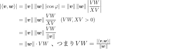
もし
![]()
注意:ドット積は双線型形式なので、以下の線型性の役に立つ表現もできます。
SVMがどの線を描いたら一番いい?
SVMがデータを二つのグループに分けるための線といえば、次の問題は、機械学習モデルはどの線を描いたら一番適当ですか?新しいデータ点が間違ったグループに割り当てられる可能性を減らすために、両方のグループからできるだけ離れた線(図4の点線)を選択するように、モデルに指示を与えたいですね。けれども、線の素顔が
図4 描きたいのは真ん中の線。右の線を選んじゃったら円の中の緑色の点は、右グループではなく左グループに入れられてしまう
信用性
一番適当な線を探す数学的な論理
今のチャレンジは「どうやって w と c を選ぶ?」ですね。データサイエンスを勉強した事がある方は絶対に信じている二つの真理が:
- 二本の目安線の分離は
- 機械学習モデルに与える指示は
最小化の条件は
では、今回の最後の難題は、上に挙げた真理は本当かどうかを確認するということです。例えば、「二つのデータ点のグループがよりよく分離されていること」が欲しければ、どうして真理が最小化をしてと書いていますか?ドット積で解明しましょう。
図5 「二つのデータ点のグループがよりよく分離されていること」「二本の目安線の分離を最大化」「オレンジ色の分離を最大化」、見た目で、全部も相当問題だけど、なぜ
図5には、左と右は二本の目安線
右の目安線のどこかに指しているベクター p と左の目安線のどこかに指しているベクター q を書きます。それで、 p が指しているポジションは任意ですが、あのポジションは目安線にありますので、
次は、二本の目安線の分離を最大化、またはオレンジ色の分離 L を最大化するために、 L を数えるのが必要です。(注意:L > 0)けれども L は p – q を w に投影した長さです!(どうぞ図5を図3にお比べ下さい。元々、私は図3を作るのに図5から描き始めたもんだ)
w は単位ベクターの
では、最後に、L の分離の最大化と
ちなみに、 p と q が指しているポジションは任意のお陰で、二本の目安線のどこかを選んでも、以上の論理が使えるので、二本の線は全体が上の議論に従っています。結果: は機械学習モデルに与える指示です。すると、将来銀行である読者様は、SVMのお陰で自動的に新しい顧客の信用性が分けられるようになります!
最後に
今回の記事で紹介してみたのは
- SVMとは?
- SVMを使う例
- ドット積とドット積の役に立つ表現
- SVMの二つの真理:
1二本の目安線の分離は
2機械学習モデルに与える指示は - 真理の本物の数学的な理
けれども、興味を持っていらっしゃる読者でしたら、今回仕入れた事の上に探求できるアイデアはまだまだあります。例えば、訓練データは簡単な線で分けられないとしたら、どうすればいいでしょうか。斉次多項式の積分変換を使ってみたら如何ですか。
そして、最後の証明には、
References 参考文献
Maitra, D. S., Bhattacharya, U., & Parui, S. K. (2015). CNN based common approach to
    handwritten character recognition of multiple scripts. 2015 13th International
    Conference on Document Analysis and Recognition (ICDAR), 1021-1025.
    https://doi.org/10.1109/icdar.2015.7333916

Meyer, D., Leisch, F., & Hornik, K. (2003). The support vector machine under test.
    Neurocomputing, 55(1-2), 169-186. https://doi.org/10.1016/S0925-2312(03)00431-4

van den Burg, G. J. J., & Groenen, P. J. F. (2016). GenSVM: A Generalized Multiclass
    Support Vector Machine. Journal of Machine Learning Research, 17(2016), 1-42.
- Tweet
-

 2024/04/23
 2024/03/26
 2024/02/27
 2024/02/23
 2024/02/09
 2024/02/02
 2024/01/23
 2024/01/12